Conditioning: The Soul of Statistics

Before delving into the concept of conditioning, it's crucial to understand probability, the foundation upon which statistical reasoning is built. You've likely heard that the probability of getting heads when flipping a fair coin is 0.5. But what does this 0.5 really mean? One interpretation is that if we flip the coin n times, we expect heads to appear in half of those flips. This is the frequentist interpretation of probability: the long-term frequency over a large number of repetitions of an experiment.

However, some experiments are non-repeatable or cannot have a large number of repetitions. For instance, consider U.S. presidential elections, which occur only once every four years. When we say, "The probability of Donald Trump getting elected is 0.6," we can't rely on a frequentist interpretation. In cases like the election example, the Bayesian interpretation becomes more appropriate. A probability of 0.6 for Trump's election reflects our degree of belief that he will win. It suggests our belief in Trump's victory is stronger than our belief in Biden's victory.

Conditioning is not only the cornerstone of statistics but also a fundamental aspect of human evolution. As we evolve, we continuously update our beliefs in light of new evidence. Let's consider an example to illustrate this concept: Imagine we're trying to determine the probability of a man being a salesman. Without any specific information about the individual, we might estimate this probability based on the general prevalence of salesmen in the male population. Let's say this initial estimate is 0.2 or 20%. In statistical terms, we call this our prior probability.

Now, let's say we gather more information about this man he wears the suit most days and spends 90% of his time talking to people. With this new information, how does our assessment change? You might now estimate the probability of him being a salesman as much higher, perhaps 0.7 or 70%. This updated probability is what we call the posterior probability - the probability we form after considering new evidence. What we've just described is the essence of conditioning. We've updated our belief about the man being a salesman after receiving new, relevant information. This process of updating beliefs is at the heart of both statistical reasoning and human cognitive development.

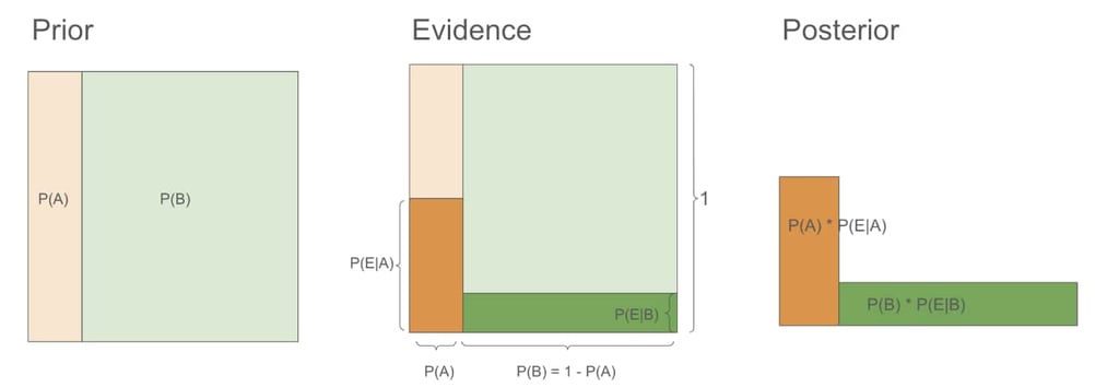
Now let's visualize the process.

What happens here essentially is our prior probability represented by the light orange and light green area got reshaped to the posterior probability represented by the dark orange and green area after the new evidence emerged. Below is the detailed illustration:

• Prior: Imagine a square with a side length of 1. This square represents our entire probability space (100%). Within this square: The light orange area represents P(A): the prior probability of the man being a salesman (0.2 or 20%), The light green area represents P(B): the prior probability of the man not being a salesman (0.8 or 80%).

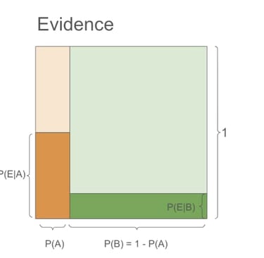
• New Evidence: Let's call our new evidence E (wears a suit, talks to people frequently). When the man is a salesman, the probability of observing our new evidence is high, around 0.9. We can write it as P(E|A) = 0.9. In our visualization, this is represented by the height of the dark orange area. When the man is not a salesman, the probability of observing our evidence is quite low, around 0.1. We can write it as P(E|B) = 0.1, represented by the height of the dark green area.

• Posterior: the posterior probability of P(A), which we can write as P(A|E) meaning the probability of the man being a salesman given the new evidence. It's the ratio between the dark orange area and the sum of the dark orange area and dark green area.

The process described above is known as Bayes' Rule, which is quite famous in statistics. I find the odds version of Bayes' Rule to be more handy. Essentially, the posterior odds are the product of the prior odds and the Bayes factor. The Bayes factor is the ratio between P(E|A) and P(E|B).